Analysis of conformational states in adaptive molecular dynamics simulations

Adaptive molecular dynamics (MD) simulation is a technique used to explore the vast and complex conformational space of proteins. Where traditional MD simulations may get “stuck” in local energy minima, failing to capture rare structural transitions, adaptive sampling overcomes this by running multiple shorter simulations in parallel. After each batch of simulations (called an epoch), the simulation data is analyzed on-the-fly, and new starting points (seeds) for the next round of simulations are adaptively selected based on specific metrics (e.g., distances, angles, mean deviation, etc.). This encourages the exploration of less-visited yet important regions of the protein’s energy landscape. All simulations from all epochs are then studied to assess changes or transitions in the conformations and other properties of the simulated molecular system. One of the approaches used to aid with this analysis is Markov state model (MSM) analysis [1], which clusters the spatial conformations observed during the simulation into similar states and characterizes the transitions between them.

In this challenge dataset, the method is applied to assess the effects of the ongoing phase 3 therapeutics tramiprosate (TMP) and its metabolite 3-sulfopropanoic acid (SPA) on the disordered Aβ42 peptide involved in Alzheimer’s disease [2]. First, molecular dynamics trajectories were generated using adaptive sampling MDs. Then, using the VAMnets approach [3], ensembles of MSMs were learned for each molecular system (Aβ42, Aβ42 + TMP, and Aβ42 + SPA) using unsupervised machine learning to cluster conformations and analyze transitions between different conformational states.

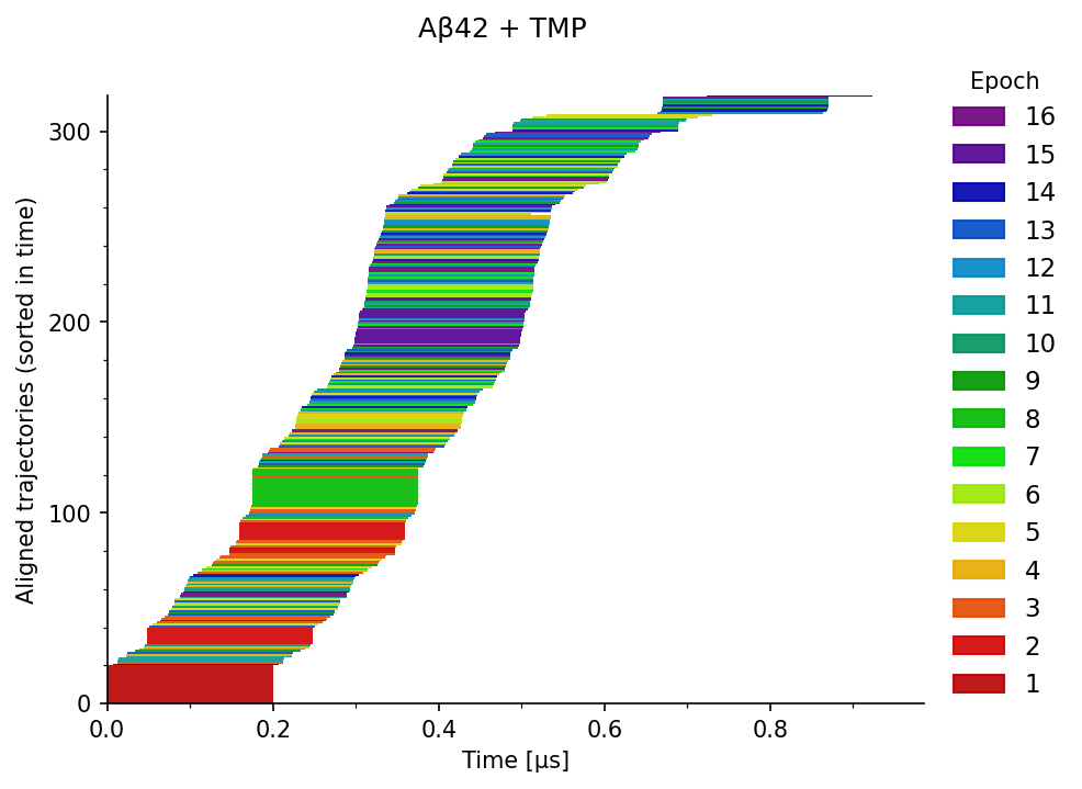
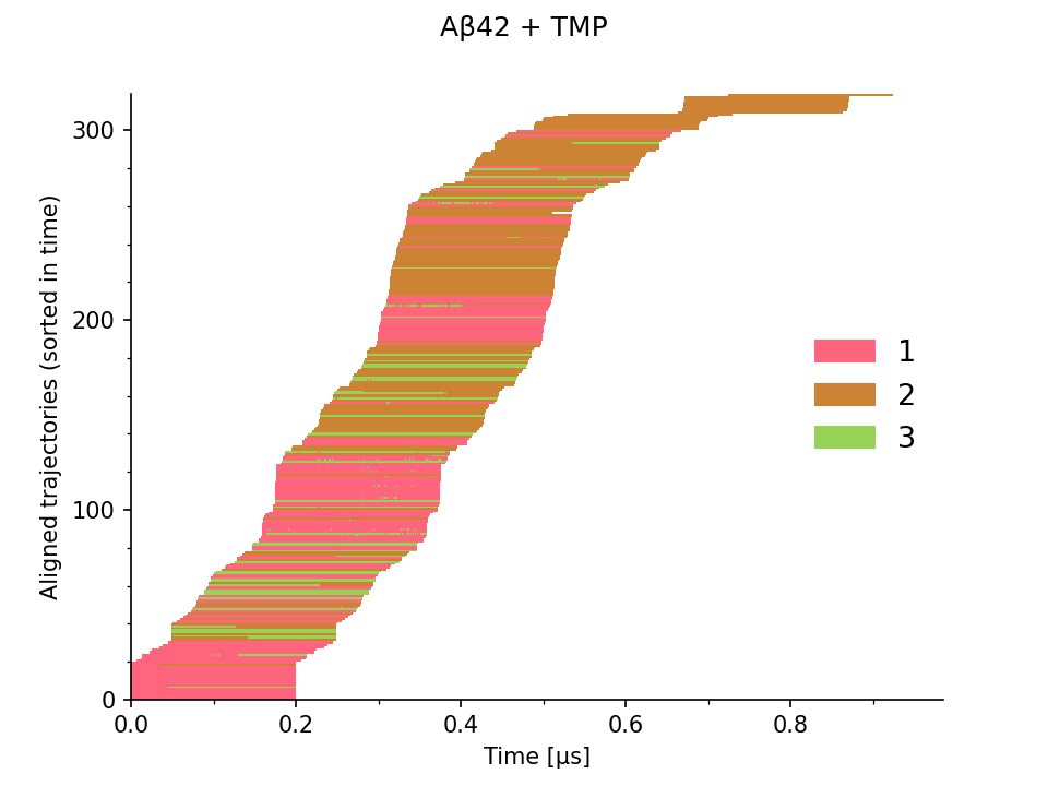
The domain experts explored this data via the following series of static charts and a simple interactive visualization. Figure 1 illustrates the distribution of the simulations over time, where each row corresponds to one MD simulation, aligned based on the time of its starting frame. On the left, the color indicates their corresponding epochs, and on the right, the assigned conformation states. It provides an overview of the temporal coverage of the sampling.

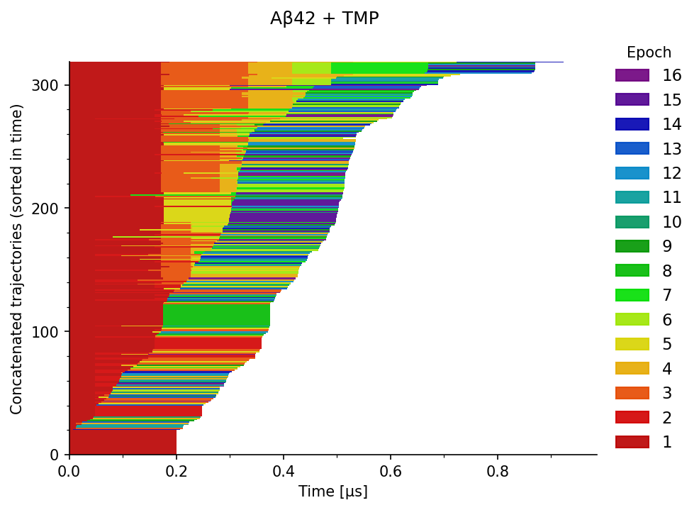
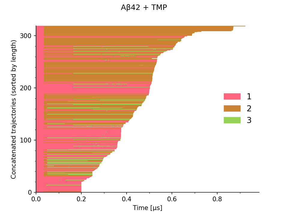
Figure 1: Distribution of the simulations over time. Each row corresponds to one MD simulation. Left: colored by epochs. Right: colored by the assigned conformation states.

The trajectories can be concatenated by joining simulations from different epochs at respective time frames (seeds) into longer continuous trajectories, as illustrated in Figure 2.

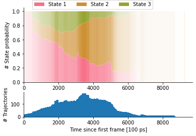
Figure 2: Concatenated trajectories. Left: colored by epochs. Right: colored by the assigned conformation states.

The overall proportions of learned Markov states in the entire ensemble can then be assessed as shown in Figure 3. Here, the opacity encodes the number of trajectories at the corresponding time (X axis), the color indicates the assigned state, and the Y axis shows the proportion of trajectories with the given Markov state.

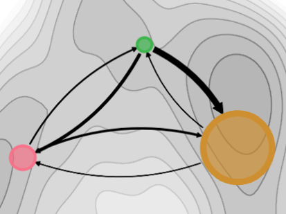
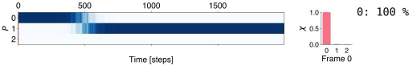
Figure 3: Top: Overall proportions of learned Markov states. Bottom: Total number of trajectories at the corresponding time (X axis).

Finally, the experts can interactively view the individual MD trajectories and observe how the molecular systems transition between individual states. This is done in a visualization (Figure 4) consisting of (a) a 3D view depicting the conformation of the molecule at a selected time point, (b) the conformation landscape view with a Markov state flow graph (here, each node corresponds to one identified state, the size of the node indicates the prevalence of the state in the entire ensemble, and the thickness of the edges indicates the transition probability) overlaid over the free energy projection (grayscale map), and (c) a timeline overview that indicates the currently selected timeframe and the state probability (each row corresponds to one state and the opacity indicates the state probability). The image below shows the simulation in the first frame, where the system is in state 0 (pink). During the interactive viewing of the trajectory, a point on the free energy landscape (b) would indicate the position of the current frame within the landscape.

Note that this last visualization (Figure 4) also includes data that are not part of this challenge. Namely, the free energy depicted in Figure 4 (b) is not provided. Furthermore, the state assignments are binary (i.e., each timeframe is assigned a single state rather than a probability of a state as indicated in Figure 4 (c)). However, the visualization can serve as an inspiration for the challenge submissions.

Figure 4: Interactive visualization of a trajectory. (a) 3D view of the molecule conformation. (b) Confirmation landscape view with a Markov state flow graph overlaid over the free energy projection. (c) Timeline overview.

Tasks

While the visualizations described above are very useful, they are limited to static summaries or interactive viewing of a single trajectory. However, the domain experts are interested in exploring the Markov states, conformations, and transition patterns across entire ensembles of trajectories and reasoning about the observed behavior. There is already a significant body of work on molecular dynamics visualization that can serve as an inspiration [4,5,6], but it does not fully address the needs of this analysis.

We thus challenge you to address one or multiple of the following tasks:

T1: Provide a better overview of the simulation ensembles. This can include designing completely novel visualizations or proposing interactions to enhance existing visualizations. For example, consider how to improve an overview of Markov state transition patterns, transition rates, and conformation landscape in summary or over time.
T2: Interactive grouping and comparison. Support interactive exploration of the data. Instead of focusing on the interactive visualization of a single trajectory, focus on the analysis of transition patterns in groups of trajectories. For example, support grouping of trajectories (including concatenated trajectories) with similar behavior or temporal alignment of trajectories based on state transitions. Consider visualization and interaction methods to aid comparison of trajectories within and between clusters or even between different systems (e.g., simulations with TMP and simulations with SPA - see data description). So far, the experts have compared the data using statistical methods and side-by-side comparison of static figures. Can this be improved?
T3: Support reasoning. Which conformational changes are responsible for Markov state assignment? Which frame, or rather multiple frames, are most representative of a Markov state? Which amino acid residues are interacting (i.e., in close proximity) with each other or with other molecules (i.e., TPM, SPA) in different Markov states? Where are those interactions happening? Incorporate additional measures, such as residue interactions or root-mean square deviation (RMSD) of atomic positions, and connect abstract and spatial representations to support reasoning about state assignments and behavior of the molecules.

Note that while some of the tasks involve the design of an interactive visualization system, we also welcome submissions with a smaller scope, such as sketches of novel visualizations and prototypes that do not have to be fully developed.

Data

The data for the challenge comes from a study assessing the effects of drug candidates on disordered biomolecules [2], consisting of simulations of three systems:

Free Aβ42 peptide - ZS-ab2
Aβ42 peptide with tramiprosate (TPM) - ZS-ab3
Aβ42 peptide with 3-sulfopropanoic acid (SPA) - ZS-ab4

Trajectories

The full data can be found at: https://data.ciirc.cvut.cz/public/projects/2023CoVAMPnet/

From this data, you will need the folder trajectories, which contains the simulated trajectories. The remaining folders are not necessary for the challenge. In the trajectories folder, you will find three subfolders, each for one of the simulated systems. Each system was simulated over 16 epochs, and each epoch consisted of 20 simulations lasting up to 2000 frames (some simulations stopped early and are thus shorter). Each system folder contains the PDB file defining the structure of the molecules and simulation folders with .xtc file encoding the MD trajectory (the format is widely supported in visualization and analysis tools such as VMD, MDAnalysis, and MDTraj). The simulation folder names adhere to the following convention: e<epochID>s<simulationID>_e<startEpochID>s<stratSimulationID>p0f<startFrameID>
where startEpochID, stratSimulationID, and startFrameID indicate the simulation and frame at which the new simulation starts.

State assignments

In addition to the trajectories, you will need state assignments. While these can be extracted from the full data, we provide a preprocessed version for easier matching with trajectories here: https://gitlab.fi.muni.cz/visitlab/bio-medvis-challenge-2026/

This repository contains three folders, one for each system. In each folder, you will find several files. Most importantly, the state assignments can be found in the files zsabX_statesY.txt, where X denotes the system and Y=2,3, or 4 represents the number of states in the Markov state model parametrization (in each parametrization, the conformations were clustered in 2,3, or 4 states, respectively). The format is the following:
Name_of_the_simulation : <list_of_states_for_each_frame>
For example:
e10s5_e5s11p0f1123: 0,0,0,0,0,0,0,0,0,0,0,0,2,0,0,0,2,2,2,0,0,0,2,2,2,2,2,2,0,2,2,2,0,2,2,...
means that the first 12 frames in the trajectory from simulation 5 in epoch 10 are assigned Markov state 0, the next one has Markov state 2, the next three have Markov state 0, the next three have Markov state 2, etc.

The remaining files contain the following information:

zsabX_names.txt - list of simulated trajectories
zsabX_order.txt - simulations ordered in time; each row has the following format:
timestep_of_simulation_start : name_of_the_simulation
zsabX_concatenated.txt - concatenated trajectories; each paragraph contains a list of simulations concatenated into a single trajectory, where each row denotes the simulation and its respective timeframes used in the concatenated trajectory in the format:
timestep_start - timestep_end : name_of_the_simulation
For example:
0-1759: e1s4_0
0-1226: e5s6_e1s4p0f1759
0+: e15s11_e5s6p0f1226
means that the concatenated trajectory consists of the first 1759 frames of simulation e1s4_0, followed by the first 1226 frames of simulation e5s6_e1s4p0f1759, and finally by all frames of simulation e15s11_e5s6p0f1226. Note that the chaining can also be derived from the names of the simulation folders.

The implementation of the system used to obtain this data, along with some of the visualizations, can be found here: https://github.com/KoubaPetr/CoVAMPnet/

Acknowledgment

This challenge was prepared in collaboration with researchers from Loschmidt Laboratories, Department of Experimental Biology and RECETOX, Faculty of Science, Masaryk University, and Czech Institute of Informatics, Robotics and Cybernetics, Czech Technical University in Prague, who kindly provided the data and expertise.

[1] Scherer, M. K., Trendelkamp-Schroer, B., Paul, F., Pérez-Hernández, G., Hoffmann, M., Plattner, N., … & Noé, F. (2015). PyEMMA 2: A software package for estimation, validation, and analysis of Markov models. Journal of chemical theory and computation, 11(11), 5525-5542. https://doi.org/10.1021/acs.jctc.5b00743

[2] Marques, Sérgio M., et al. CoVAMPnet: comparative Markov state analysis for studying effects of drug candidates on disordered biomolecules. JACS Au, 2024, 4.6: 2228-2245. https://doi.org/10.1021/jacsau.4c00182

[3] Mardt, A.; Pasquali, L.; Wu, H.; Noé, F. VAMPnets for Deep Learning of Molecular Kinetics. Nat. Commun 2018, 9 (1), 5. https://doi.org/10.1038/s41467-017-02388-1

[4] Ulbrich, P., Waldner, M., Furmanová, K., Marques, S. M., Bednář, D., Kozlíková, B., & Byška, J. (2022). sMolBoxes: Dataflow model for molecular dynamics exploration. IEEE Transactions on Visualization and Computer Graphics, 29(1), 581-590. https://doi.org/10.1109/TVCG.2022.3209411

[5] Belghit, Hayet, Mariano Spivak, Manuel Dauchez, Marc Baaden, and Jessica Jonquet-Prevoteau. “From complex data to clear insights: visualizing molecular dynamics trajectories.” Frontiers in Bioinformatics 4 (2024): 1356659. https://doi.org/10.1016/j.jmb.2018.09.004

[6] Kozlíková, B., Krone, M., Falk, M., Lindow, N., Baaden, M., Baum, D., … & Hege, H. C. (2017, December). Visualization of biomolecular structures: State of the art revisited. In Computer Graphics Forum (Vol. 36, No. 8, pp. 178-204). https://doi.org/10.1111/cgf.13072

Questions?

Please feel free to send any questions to: biovis_challenge@ieeevis.org.

Chairs of the Bio+MedVis Challenge @ IEEE VIS 2026:

Katarina Furmanova, Masaryk University, Czech Republic
Daniel Haehn, University of Massachusetts Boston, USA
Robert Krueger, New York University, USA